
Practical guide · Trial Planner + R · Synthetic data
How to plan a trial with a binary response outcome
From a clinical question to a defensible sample size: expected response rates, an important effect, power, allocation and missing outcomes.
Learning objective: complete a Trial Planner scenario, reproduce it in R and explain why the answer changes when assumptions change. The main example assumes a 25% control response and a 40% treatment response. These are teaching assumptions, not claims about a real treatment or population.
Open Trial Planner · Read the SatraGO news article behind this guide · Download code and data
1. Define what counts as a response
Imagine a parallel trial with individual randomization to an experimental treatment or control. Each participant has an assessment at week 24 and a binary outcome: response or no response. Response is beneficial. Before seeing the results, investigators specify the clinical criterion, assessment window and rules for rescue therapy, treatment discontinuation and death. These decisions form part of the scientific question and should not be improvised during analysis.
The target population needs a sufficiently precise description for the assumed response rates to be meaningful. The analysis unit is the person, and observations must be independent across participants. Our teaching comparison is the marginal probability difference, RD = pT − pC. We do not adjust for centres or covariates, and we do not model repeated measurements. A real protocol may require those extensions.
Two thresholds must remain distinct. The individual response criterion determines who is a responder. The between-group target difference specifies the alternative under which we want power. Here, 15 percentage points is an illustrative working assumption. We do not claim it is a validated minimal clinically important difference for a particular disease.
2. Write the assumptions before opening the calculator
| Decision | Assumption |
|---|---|
| Control response | 25% |
| Treatment response | 40% |
| Target effect | RD +15 percentage points; RR 1.60 |
| Test | Equality of risks; two-sided alpha 0.05 |
| Target power | 90% |
| Treatment:control allocation | 1:1 |
| Common fraction without a usable outcome | 10% |
Power is evaluated under pC=0.25 and pT=0.40. The null hypothesis remains H0: pT=pC. The 15-point target is not converted into a margin that the estimate must exceed. Designing to detect a difference and demonstrating that a difference exceeds a clinical threshold are different statistical objectives.
Power of 90% is a probability of rejection under that alternative and procedure, approximate in this case. It is not a 90% probability that the treatment works, or that the development programme succeeds. Choosing a one-sided or two-sided test requires a prospective justification; it should not depend on which option gives a smaller sample size.
3. Solve it in Trial Planner and understand rounding
- Open Trial Planner in English and select sample-size calculation.
- Enter control 25%, treatment 40%, power 90%, alpha 0.05, a two-sided test and 1:1 allocation. Select “Favourable event” under event interpretation: the event here is a response.
- Check the result with 0% missing first: 203 evaluable participants per group, 406 total.
- Change the common fraction without a usable outcome to 10%: randomize 226 per group, 452 total.
- Keep the inputs and method with the answer; a total alone does not document the design.
For 1:1 allocation, each block contains one person in each arm. With 203 information blocks and 90% retention, the calculation is ceiling(203/0.90)=226 randomized blocks. Arms are not rounded independently in a way that breaks the allocation. The answer is the minimum integer reaching the target within this method, rather than a guarantee of exact finite-sample power.
This adjustment compensates planned information counts under common, conditional retention. It does not integrate power over all possible random realizations of missingness. It also does not recommend excluding participants with incomplete data from the analysis. The estimation strategy needs a separate specification.
4. Which method produces the number?
Trial Planner uses a normal approximation for two independent proportions without a continuity correction. It combines a variance under equal risks with a variance under the alternative. For a two-sided test, it includes rejection probabilities in both tails. The downloadable script exposes these operations with qnorm and pnorm, rather than hiding a different formula behind the same label.
p̄ = (nTpT + nCpC)/(nT+nC)
V0 = p̄(1−p̄)(1/nT+1/nC)
V1 = pT(1−pT)/nT + pC(1−pC)/nC
For d=pT−pC and z=Φ−1(1−α/2): power = Φ((d−z√V0)/√V1) + Φ((−d−z√V0)/√V1).
The search increases the number of allocation blocks and locates the first integer reaching the power target. For balanced allocation, power is also checked against stats::power.prop.test(strict=TRUE). In that function, n is the number per arm and strict=TRUE retains both tails. Agreement checks this particular procedure, not every possible sample-size method. Official R documentation.
The approximation can differ from rejection probabilities when the test is applied to actual binomial counts. Extreme probabilities or small cells require scrutiny and may call for exact methods or simulation. A small-expected-cell warning is useful, but exceeding a particular count does not certify that an approximation is adequate.
5. Examine nine scenarios, rather than one number
The table holds two-sided alpha at 0.05, power at 90%, allocation at 1:1 and the fraction without a usable outcome at 10%. Control response and assumed RD vary. Each row represents a different hypothetical future trial. These answers are neither confidence intervals nor probabilities assigned to the scenarios.
| Control | Treatment | RD (pp) | Evaluable per arm | Total to randomize |
|---|---|---|---|---|
| 15% | 25% | 10 | 335 | 746 |
| 25% | 35% | 10 | 440 | 978 |
| 35% | 45% | 10 | 503 | 1118 |
| 15% | 30% | 15 | 161 | 358 |
| 25% | 40% | 15 | 203 | 452 |
| 35% | 50% | 15 | 227 | 506 |
| 15% | 35% | 20 | 97 | 216 |
| 25% | 45% | 20 | 118 | 264 |
| 35% | 55% | 20 | 128 | 286 |
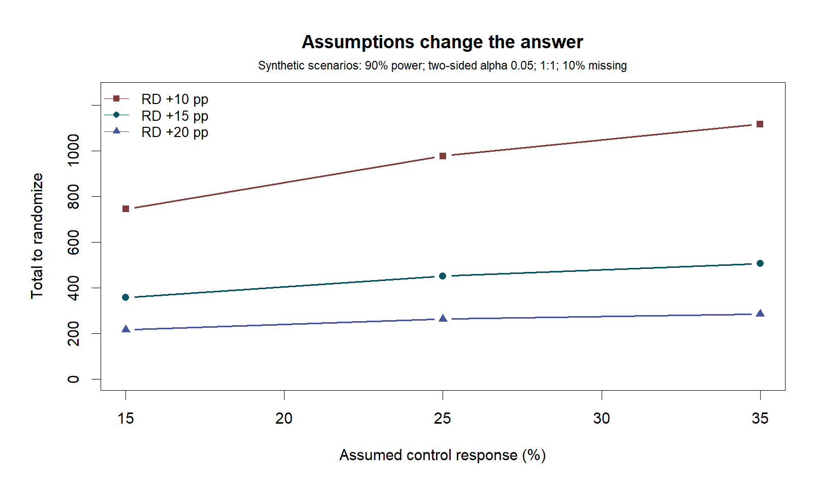
At a 25% control response, changing the assumed RD from 20 points to 10 points increases the randomized total from 264 to 978. This is not a calculator failure: the aim is to detect a smaller signal against variability. Choosing the most favourable scenario to meet a budget changes the question the trial will be able to address.
When varying the baseline response, specify which effect is held fixed. With a fixed 15-point RD, control responses of 15% and 35% imply treatment responses of 30% and 50%. With RR fixed at 1.60, the corresponding treatment rates would instead be 24% and 56%. These are different alternatives and should not be mixed in a chart without explanation.
A sensitivity analysis makes the consequences of assumptions visible without pretending to know which scenario will occur. Selecting a probability distribution for those assumptions and averaging success probabilities would be another task. It requires a justified distribution and a stated decision rule; the scenario table does not provide that assurance calculation.
6. Unequal allocation and unavailable outcomes
Under the base response assumptions, 2:1 allocation requires 154 evaluable control participants and 308 treatment participants. With 10% missing, randomize 172 and 344, for a total of 516. This recruits more people than the 452 total under 1:1 allocation. Unequal allocation may have clinical or operational reasons, but its information cost should be visible.
With 1:1 allocation, increasing expected missingness from 10% to 20% raises the randomized total from 452 to 508. That arithmetic does not correct bias. If people without a measurement systematically have worse outcomes, restoring the same number of observations does not solve the problem. Follow-up, reasons for missingness, analysis and sensitivity should be planned.
MCAR describes missingness independent of relevant data; MAR makes the corresponding independence conditional on observed data; MNAR allows dependence on unobserved values. MAR cannot be established merely by examining complete records. The assumption needs justification and, when material, sensitivity analyses. Intercurrent events such as rescue therapy or discontinuation also need a strategy aligned with the estimand, following ICH E9(R1).
7. Reproduce and explore in R
Download the script, save it to a folder and open it in RStudio. No package installation is needed: it uses base R, stats, graphics and grDevices. Choose the output directory explicitly. The following commands create the CSV files, figures and session record:
source("binary-planning.R")
run_exercise("results")
plan_binary(0.25, 0.40, missing = 0.10)
plan_binary(0.25, 0.40, allocation = c(2, 1), missing = 0.10)
stats::power.prop.test(n = 203, p1 = 0.25, p2 = 0.40,
  sig.level = 0.05, alternative = "two.sided", strict = TRUE)
The 400-participant CSV contains a synthetic identifier, arm and response, generated with seed 20261019. This is a separate exercise: observing one sample is not the same as treating its generating probabilities as newly known. The analysis file applies prop.test(correct=FALSE) and reports an estimate, interval and test for those synthetic data. It does not reproduce SatraGO's adjusted analysis.
This realization contains 63 responses among 200 control participants (31.5%) and 78 among 200 treatment participants (39.0%). The observed difference is 7.5 points, with an approximate 95% interval from −1.83 to 16.83 and p≈0.116. It illustrates sampling variation: high prospective power does not guarantee significance in a particular realization. We do not calculate “observed power” to interpret this result.
The script also exports the published SatraGO estimates as an aggregate summary file, clearly separated from the synthetic participant records. The clinical figures use the published 95.03% intervals rather than creating new intervals from rounded percentages. Session information records the version actually executed, supporting an auditable reproduction.
8. Four exercises with worked answers
1. Why is “we expect twice the response” insufficient?
Baseline risk changes the alternative and the variance. Moving from 5% to 10% and from 20% to 40% both give RR=2, but their absolute differences are 5 and 20 points. State both response probabilities and justify their plausibility before calculating.
2. Does 203 per group mean we should randomize 406?
Only under the assumption that all usable outcomes will be available. With 10% commonly missing, ceiling(203/0.90)=226 per group, 452 total. Inflation neither specifies a missing-data analysis nor removes possible bias.
3. Do p≈0.086 and p≈0.0077 imply different treatment effects?
The labels cannot establish that conclusion. In the synthetic example of independent estimates of 12±7 and 16±6 points, their difference is 4 points, with standard error 9.22, an approximate 95% interval of −14.1 to 22.1 and p≈0.664. Equivalence has not been established either.
4. Should we copy SatraGO's largest observed difference?
Not automatically. Review population, response definition, assessment time, estimand and method; justify an important and plausible target and explore uncertainty. Post hoc power computed from the observed effect does not supply a new, independent measure of evidence.
9. Downloads and the next decision
Before placing a number in a protocol, document the rationale for the rates, who considers the difference important, the estimand, the main analysis and sensitivity analyses. DELTA² provides a framework for justifying a target difference. This guide covers one binary outcome, two independent groups and a single final superiority test. Survival, non-inferiority, clustering, interim analyses and multiplicity require a separately specified design.
Return to the full SatraGO news article to reconnect the exercise with the clinical context. Keep three questions separate: what was observed, what is inferred under assumptions, and which scenario is being planned for the next study.