
Practical guide · Synthetic data
Kaplan–Meier, step by step
Read a survival curve, understand censoring and reproduce the result with a fictional clinical case.
01 · The clinical case
The clinical case
300 fictional patients, 150 in A and 150 in B. What probability of being alive at 12 months from diagnosis do we estimate in each group?
- Time zero
- Cancer diagnosis
- Event
- Death from any cause
- Maximum follow-up
- 24 months
A/B are exercise labels. The numbers represent neither a real clinical population nor treatments.
Case definition and learning objectives
By the end, you will be able to estimate and interpret survival at 12 months, understand the number-at-risk table and reproduce the calculation in R.
- Read a Kaplan–Meier curve, its censoring marks and confidence intervals.
- Distinguish survival probability from the number of people still at risk.
- Obtain the same results with Survival Lab and the
survivalpackage in RStudio using the same data.
Imagine a completely fictional cohort of 300 adults with a cancer diagnosis, followed for up to 24 months. A and B are two groups defined at baseline, with 150 patients each; they are exercise labels, representing neither treatments nor validated clinical categories. We want to answer: what probability of being alive at 12 months from diagnosis do we estimate in each group?
The unit of analysis is the patient and time zero is diagnosis. The event is death from any cause. Observed follow-up ends at death, at the last contact confirming that the patient is alive if follow-up is subsequently lost, or at closure at 24 months. The latter two are right censoring: we know survival up to that time, but not what happens afterwards.
The estimand is marginal survival within each group, S(t) = P(T > t), especially S(12). Group is the only stratification factor: there is no covariate adjustment, hypothesis test or causal effect estimation. The records are simulated; the case provides context for the exercise and its numbers do not describe a real clinical population.
02 · Explore each step
Explore each step
Independent five-person example: move through the months and observe what changes with an event and with censoring. Confidence intervals are not shown.
- KM survival
- At risk immediately before
- Remaining afterwards
Crosses mark censoring; the line shows Kaplan–Meier survival.
Step calculation:
Read the explanation and complete table
| Month | At risk before | Events | Censored | KM afterwards |
|---|---|---|---|---|
| 0 | 5 | 0 | 0 | 100% |
| 1 | 5 | 1 | 0 | 80% |
| 2 | 4 | 1 | 1 | 60% |
| 3 | 2 | 0 | 1 | 60% |
| 4 | 1 | 1 | 0 | 0% |
At each event time, Kaplan–Meier multiplies survival by (1 − events/people at risk). Censoring alone does not lower the curve: the person stops contributing to later risk sets. This is the logic of the estimator introduced by Kaplan and Meier (1958).
A five-person example makes this visible: an event at month 1; one event and one censoring at month 2; censoring at month 3; an event at month 4. Survival moves from 1 to 4/5 = 0.80, then to 0.80 × 3/4 = 0.60. At month 3 it remains 0.60. The person censored exactly at month 2 is included among the four people at risk immediately before that time. The summary.survfit documentation specifies this convention.
The final event takes the estimate to zero with only one person at risk. This does not establish certainty about population survival. Intervals are pointwise, rather than a simultaneous band for the entire curve. A plateau and an interval that stays unchanged after censoring do not guarantee substantial remaining follow-up: always read the risk table.
03 · Read the result
Read the result
With the synthetic example data, we obtain:
| Group | Kaplan–Meier at 12 months | Pointwise 95% CI | At risk immediately before 12 months |
|---|---|---|---|
| A | 65.12% | 56.48–72.47% | 85 |
| B | 78.63% | 70.85–84.56% | 98 |
In A, 85/150 = 56.7% is not estimated survival at 12 months. These 85 people are still under observation and event-free immediately before that time. Kaplan–Meier uses risk sets at each event time, accounting for when follow-up ends; it therefore estimates 65.12%.
04 · Reproduce the analysis
Reproduce the analysis
In the browser
- Open Survival Lab and launch the tool.
- Set 150 people per group, event risk in A at 12 months to 0.30, HR for B versus A to 0.65, follow-up to 24 months, latent dropout probability at 12 months to 0.15, and seed to 20261008. Enter probabilities on the scale shown by each control.
- Select Simulate. Edited controls leave the previous result visible until you simulate again; downloads describe the most recently executed result.
- Inspect the step curve, censoring marks, pointwise 95% confidence intervals and risk table. The dashed curve is the generating truth, known only because the data are simulated.
- Download observed data, summary, risk table and R script. Keep the parameters to document the scenario.
View the Lab screenshot and its provenance
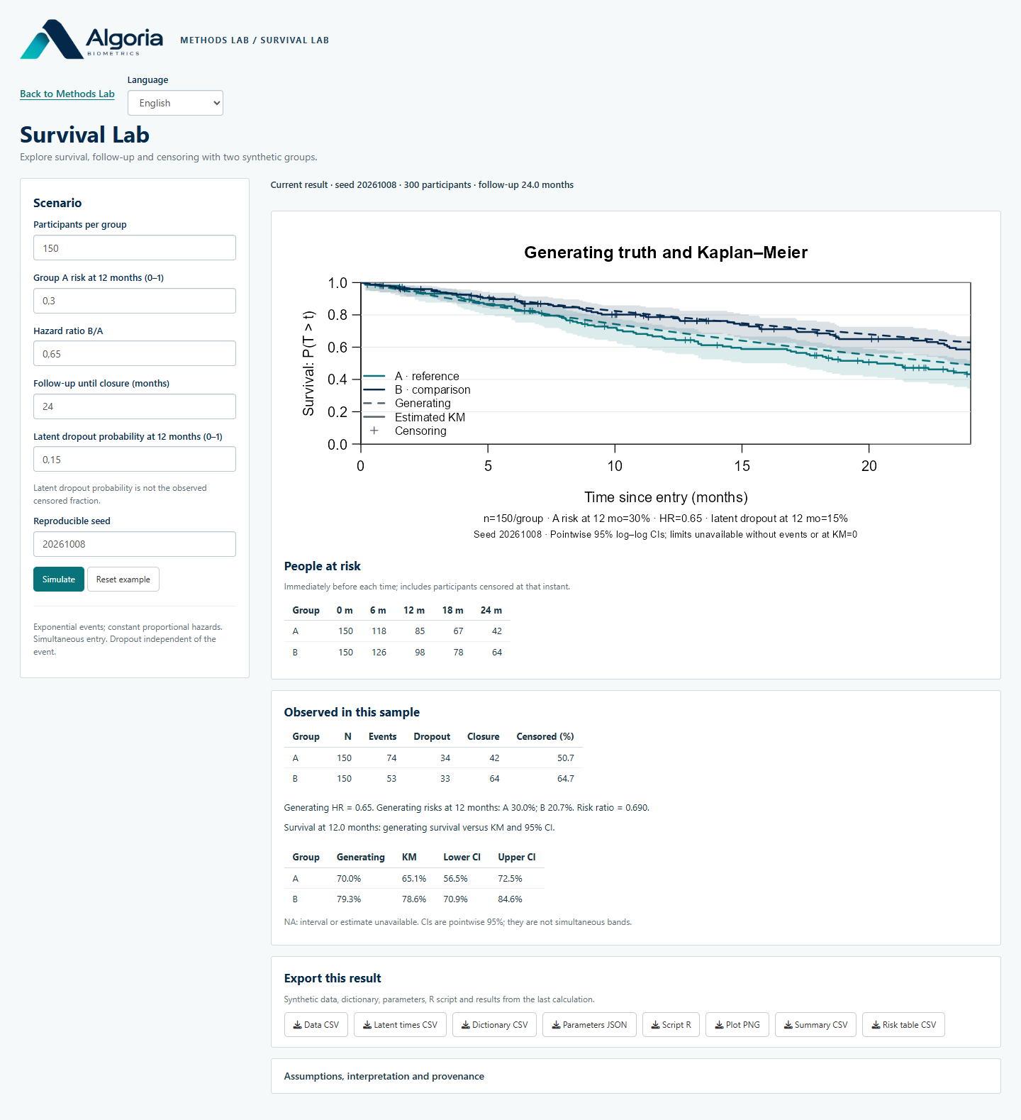
Screenshot of the local Shiny application, using the same Lab engine. Shading shows pointwise confidence intervals; dashed curves show generating survival. The on-screen summary uses one decimal place; the following table uses two.
With R / RStudio
You can run the same analysis outside the lab. RStudio is the
interface; survival is the R package that calculates
Kaplan–Meier, also used by Survival Lab. This route analyses
the same CSV without simulating the data again.
- You need R and, to follow the screenshots, RStudio. If
survivalis missing, runinstall.packages("survival")once in the R console. - Save the example CSV and the short survival script in the same folder. The CSV contains the 300 observed records from the scenario above.
- Open the script in RStudio with File → Open File. Select Session → Set Working Directory → To Source File Location so R finds the CSV without personal paths in the code.
- Select Source. The console shows S(12), confidence limits and risk counts. Plots shows the curves and censoring marks. The script validates the CSV before fitting and is specifically prepared for this synthetic example.
The core calculation is:
library(survival)

d <- read.csv("synthetic-data.csv")

d$group <- factor(d$group, levels = c("A", "B"))

fit <- survfit(Surv(time, event) ~ group, data = d,

               conf.type = "log-log", conf.int = 0.95)

summary(fit, times = 12, extend = FALSE)

summary(fit, times = c(0, 6, 12, 18, 24), extend = FALSE)
In this fictional case, event=1 represents death from
any cause; event=0, right censoring. time is
observed follow-up in months from diagnosis. We explicitly select
pointwise 95% log–log intervals, matching the Lab; the package default
is different. extend=FALSE avoids extending estimates
beyond observed follow-up. See survfit
and summary.survfit.
View the RStudio screenshot and its provenance
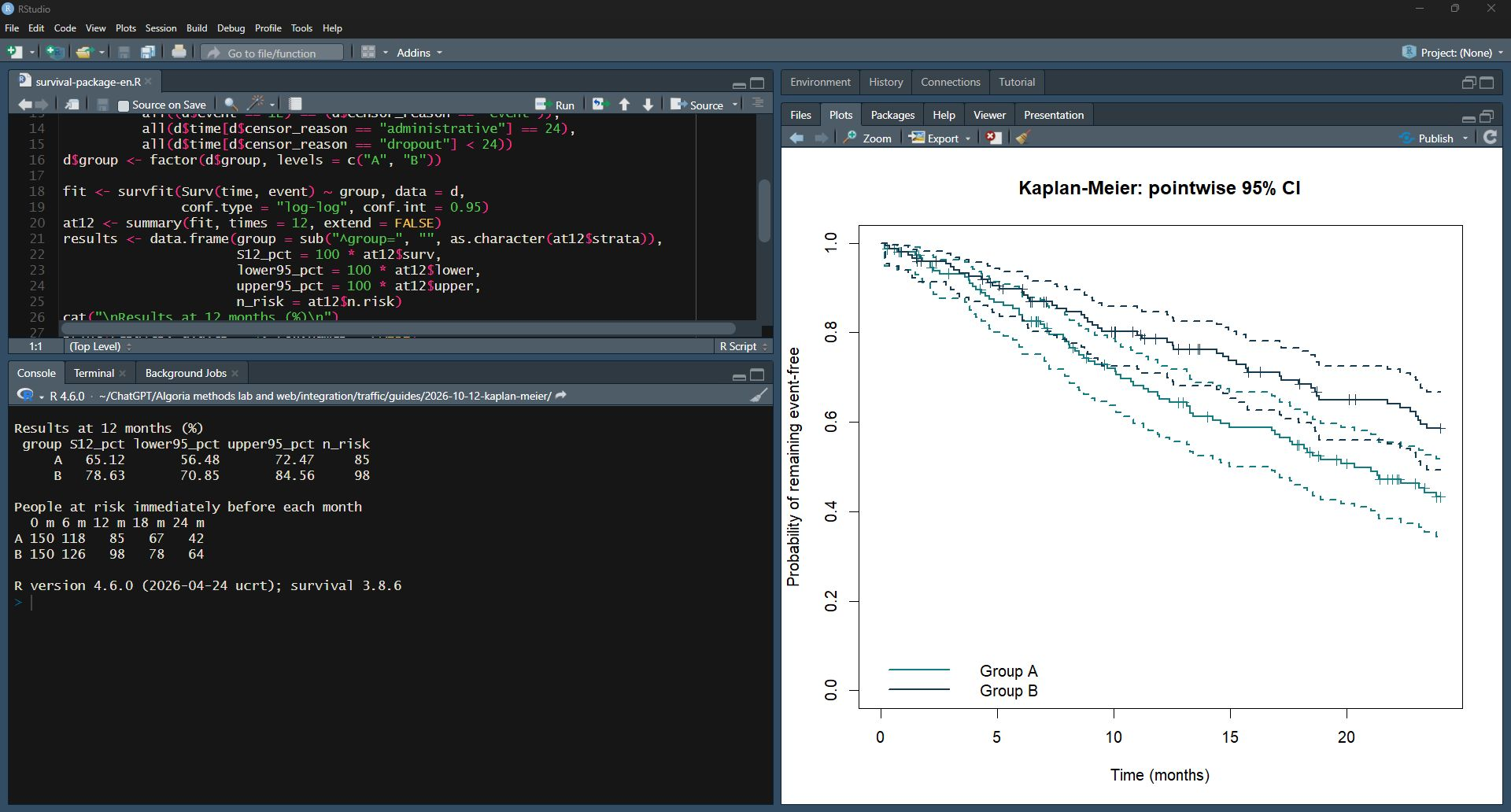
Actual screenshot of RStudio. Crosses indicate censoring; dashed lines delimit the pointwise confidence intervals. This plot does not include generating truth.
S(12), both confidence limits and every risk count at 0, 6, 12, 18
and 24 months match the Lab. The plot looks different because it uses
plot.survfit(); the estimator is the same. Versions and
numerical verification are documented in the optional technical
block.
Keep the same CSV to repeat the exact sample.
05 · Assumptions and technical detail
Assumptions and technical detail
Interpreting the case requires a clearly defined event and start of follow-up, independent patients, and censoring independent of time to death within each group. In the simulation, dropout is generated independently. In a real cohort this assumption would need justification: if patients whose prognosis worsens are more often lost to follow-up, the estimate may be biased. Consider sensitivity analyses if independence is not defensible.
Kaplan–Meier itself does not require exponential event times or proportional hazards. Competing risks, delayed entry, recurrent events and changing covariates require a different approach. This lab cannot import real data and does not include Cox, log-rank or power. Visual curve separation or overlap between their confidence intervals is not a between-group test.
Optional technical detail: simulation, counts and reproducibility
How the example is generated
The generator uses exponential events, constant proportional hazards, simultaneous entry into follow-up, independent dropout and common closure at 24 months. This is a simplified teaching scenario; it is not calibrated to a real disease or treatment.
The generator sets lambda_A = −log(0.70)/12 and lambda_B = 0.65 × lambda_A. Therefore S_A(12) = 0.70 and S_B(12) = 0.70^0.65 = 0.793074: 70.00% and 79.31%, respectively. These are simulation population values, distinct from estimates obtained in a sample. HR = 0.65 is a generating parameter, not an estimated clinical effect, and does not mean that B’s risk is 0.65 times A’s risk.
| End of observation, through 24 months | A | B |
|---|---|---|
| Event (death in the fictional case) | 74 | 53 |
| Dropout | 34 | 33 |
| Administrative closure | 42 | 64 |
These counts cover 24 months, not 12. The censored fractions are 76/150 and 97/150, including dropout and administrative closure. The 0.15 parameter describes P(latent dropout time ≤ 12); it is not the observed censored fraction. The event may precede dropout, and closure also causes censoring.
Versions and equivalence
The original reference used R 4.5.2 and survival 3.8-3. The actual RStudio screenshots use RStudio 2025.09.2+418, R 4.6.0 and survival 3.8-6. Both short exercises were checked against a fresh Lab calculation and the original reference: full curves, S(12), confidence limits and risk counts agree within tolerance 10⁻¹⁰. This check covers the stated versions, not every possible version.
The fit uses conf.type="log-log"; see survfit.formula.
Survival Lab omits log–log limits when estimated survival is 0 or 1. The
same seed with another generator does not guarantee identical records.
The Lab’s latent times explain the simulation and are not used to fit
KM.
Reproduce the simulation and the Lab plot too
Save the example R script and, if
you want to inspect the records, the
synthetic CSV. Run the script in an empty output folder, with R and
the survival package available:
Rscript --vanilla survival-guide-en.RThe standalone script is generated by Survival Lab’s existing
exporter. It creates survival-data.csv,
survival-summary.csv and survival-plot.png,
and prints the versions used. Reproducing the calculation does not
require Shiny. Output names are fixed: use an empty folder to preserve
earlier results.
This route reproduces the generator and the Lab’s plot design too. The short RStudio alternative reproduces the CSV analysis using the package’s standard plot.
06 · Solve the case
Solve the case
Choose an answer and check your interpretation. You can open the explanation for each question.
The skill you can transfer to research is defining the event and time zero, interpreting the curve, confidence intervals and risk table together, and keeping the data and code to reproduce the result. Before applying it to a real cohort, examine how groups were defined and why follow-up ended.
Continue in Methods Lab. To adapt an analysis to a study, see Longitudinal, Survival & Sensitivity Analysis.